Running the Pipeline

If you have any questions or issues, feel free to open an issue or directly email Drew Neavin (d.neavin @ garvan.org.au)

Phew, ok, now that you have prepared all of the inputs, downloaded all the materials and installed the software, you are ready to run the pipeline. All of the steps for running the softwares used for demultiplexing and doublet detection for this pipeline have been built into a Snakemake infrastructure using softwares installed in a Singularity image. Once all the softwares have run, the pipeline will also run steps to merge the results together, assign final droplet types and provide QC figures for selecting final filtering thresholds.

Ideally you would just run the pipeline and it would output all of the results. However, there are two softwares that require user input in order to ensure that the thresholds are adequate. If the thresholds are not well chosen by the software, you will have to rerun those steps before moving on. This has been built into the pipeline by ensuring that it will not move forward with merging results from multiple softwares until you have confirmed that the outputs look sufficient. We will provide examples of pools that are adequate to move forward as well as examples of pools that need further testing and thresholding before moving forward with the pipeline in the instructions below.

Note

With the implementation of newer versions of the pipeline, it is important to make sure your singularity image alignes with the version of the pipeline documentation that you are currently using. To check the version of your singluation image plase run:

singularity inspect WG1-pipeline-QC_wgpipeline.sif

which will tell you the image version you are currenlty using and, therefore, the relevant documentation for that image.

Preparing to Run the Pipeline

1. The first step is to copy the sceQTL-Gen-Demultiplex.yaml from the pipeline directory to a working directory and edit it based on your system, directories and setup

   • Snakemake uses the contents of this file for running all the steps of the pipeline

2. Then you will need to edit the contents of this file to reflect the file locations on your system

   • This file has all the parameters that you can change for the pipeline. However, most of the parameters shouldn’t require editing so we have organized them into 4 main categories:

     • File locations on your system that require your input (Requires user input)

     

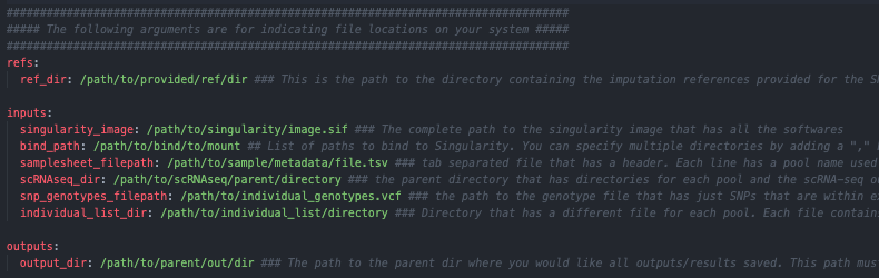
     • Parameters that more often need to be edited but are not required to be changed (Mostly includes the number of threads and amount of memory to use)

     

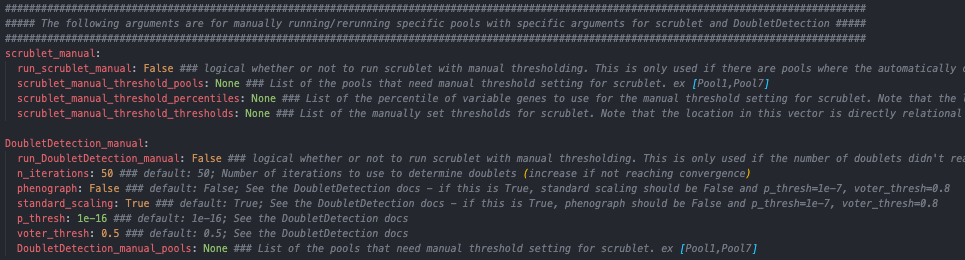
     • Parameters that will need to be changed if manual rerun of the two softwares that require user monitoring is needed (This will be addressed below after identifying what results would require manual reruns of specific pools)

     

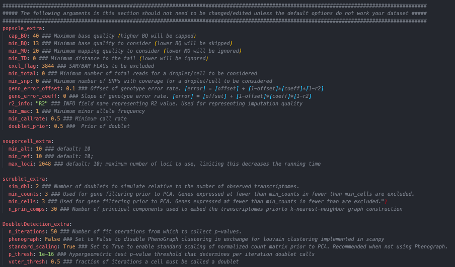
     • Parameters that usually do not need to be edited for each of the softwares (default parameters of each of the softwares - these will only need to be changed if the defaults are returning unanticipated results)

     

   • Within each of these categories, we havevalso separated the arguments for each software into separate sections for clarity

3. After you have provided the correct file locations, you are ready to run the pipeline with Snakemake but let’s define some variables that will make it easier to run and cleaner.

   • Let’s define a variable, $SCEQTL_PIPELINE_SNAKEFILE which is the location of the snakefile which is in the cloned github repository:

   SCEQTL_PIPELINE_SNAKEFILE=/path/to/WG1-pipeline-QC/Snakefile
   

   • Let’s also define a variable for the location of the edited configuration yaml:

   SCEQTL_PIPELINE_CONFIG=/path/to/edited/sceQTL-Gen_Demultiplex.yaml
   

   • Finally, let’s define a location that we would like to keep the cluster log outputs and make the directory

   LOG=/path/to/cluster/log_dir
   mkdir -p $LOG
   

   • Please keep in mind that you will have to define these variables any time you have to log back in to the cluster to run next steps if you were disconnected. Since this is a multiple day pipeline, we suggest saving each of the paths used in a file that you can source or that you can easily execute from to make starting the pipeline at the next step easier

Phase 1

Finally, we can run Snakemake. For the example, we will use the full test dataset described at the beginning. If you decide to also use this dataset, your results should be similar to what is presented here.

If you are comfortable with using Snakemake, you can skip to the Quick Run section that will have far less details than this section.

1. First let’s do a “dry run”. This will allow Snakemake to check all our files and tell us which jobs it will run (remember to activate you snakemake environment before running: conda activate wg1_snakemake):

   snakemake \
       --snakefile $SCEQTL_PIPELINE_SNAKEFILE \
       --configfile $SCEQTL_PIPELINE_CONFIG \
       --dryrun \
       --cores 1 \
       --reason
   

   • Here is an example dryrun output for one pool:

   

   • Note that the jobs: “all”, “make_DoubletDetection_selection_df” and “make_scrublet_selection_df” will only run one count regardless of the number of Pools that you have but all other jobs will run the count number of pools that are being demultiplexed (ie if 4 pools are being demultiplexed, then the count should be 4)

   • For this example, we are using the example Sample Table (#2 of Required Input) in this github repository: samplesheet.txt, which only contains one pool (called test_dataset) of 12 individuals

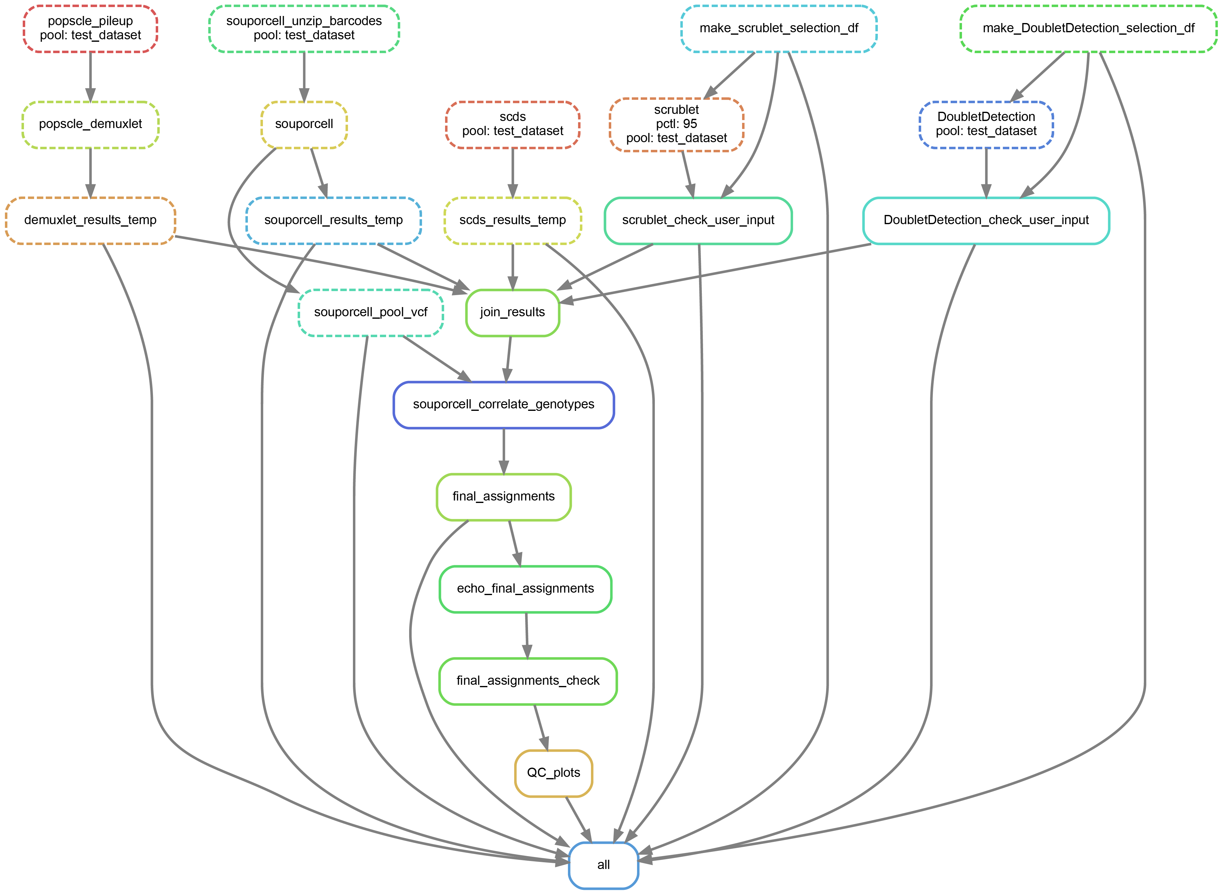
2. We can also create a directed acyclic graph (dag) showing each of the jobs that will be run and their dependency on one another:

   snakemake \
       --snakefile $SCEQTL_PIPELINE_SNAKEFILE \
       --configfile $SCEQTL_PIPELINE_CONFIG \
       --dag | \
       dot -Tsvg \
           > dag1.svg
   

   • Here’s an example of a dag for the above dry run

     

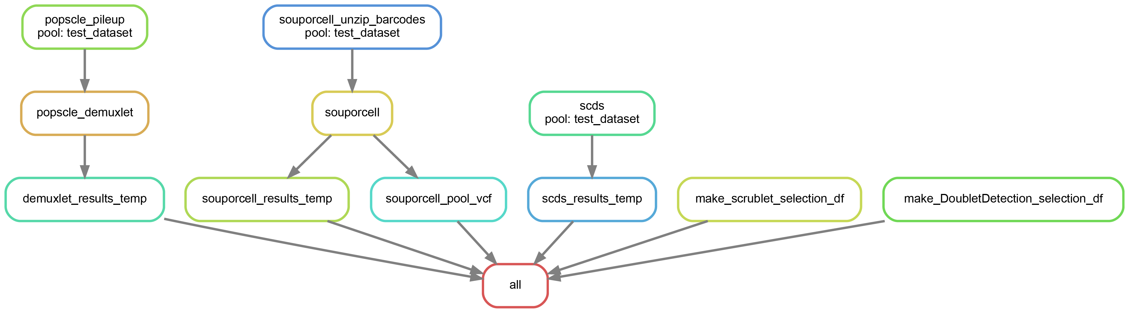
     • The name of the pool we are using in this example is “test_dataset”

     • As you can see, the jobs for each of the softwares are independent of one another

3. Next we can actually submit the pipeline so that each of the jobs are run. I don’t recommend running this pipeline locally because because it will require many parallel jobs, some of which could use upwards of 250GB of memory. Therefore, you can ask Snakemake to run each independent job as a separate cluster submission with the following code (or some variation of it depending on your system).

   Important

   If the chromosomes in your vcf are not in the same order as your bam file, you will receive an error from popscle. We have provided some instructions on how this can be fixed in the Common Errors and How to Fix Them Section.

   nohup \
     snakemake \
       --snakefile $SCEQTL_PIPELINE_SNAKEFILE \
       --configfile $SCEQTL_PIPELINE_CONFIG \
       --rerun-incomplete \
       --jobs 20 \
       --use-singularity \
       --restart-times 2 \
       --keep-going \
       --cluster \
           "qsub -S /bin/bash \
           -q short.q \
           -r yes \
           -pe smp {threads} \
           -l tmp_requested={resources.disk_per_thread_gb}G \
           -l mem_requested={resources.mem_per_thread_gb}G \
           -e $LOG \
           -o $LOG \
           -j y \
           -V" \
     > $LOG/nohup_`date +%Y-%m-%d.%H:%M:%S`.log &
   

   • A couple of notes about the above command:

     • Using nohup enables us to let the pipeline keep running when we log out of the cluster

     • To enalbe the snakemake command to be run in the background and write the output to be written to a file in your $LOG directory, we use: > $LOG/nohup_`date +%Y-%m-%d.%H:%M:%S`.log &

     • The pipeline has been setup to use more memory with each automatic rerun, which is increased linearly. This has been done so that the user does not have to manually increase and manually rerun when a job fails. Therefore, if the user has indicated that 20GB should be used with 1 thread, that amount will be used for the first run and if it fails, 40GB with 1 thread would be used, then 60GB and so on. Of course this will only happen if --restart-times is used in the snakemake command

     • There are many additional parameters that can be used by Snakemake which can be found on their website such as --resources which may be helpful for some people

     • Souporcell and popscle can take up to a day or so to run.

     • Popscle-pileup (the step before using demuxlet) also uses a huge amount of resources and will fail if it doesn’t have enough memory. We have noticed that on our cluster, popscle will core dump or stop without returning a failed signal to snakemake. In these instances, snakemake does not know that it failed and thus does not know that it has to be rerun. Therefore, the user may have to manually rerun popscle-pileup after increasing the amount of memory in the yaml file in the popscle section

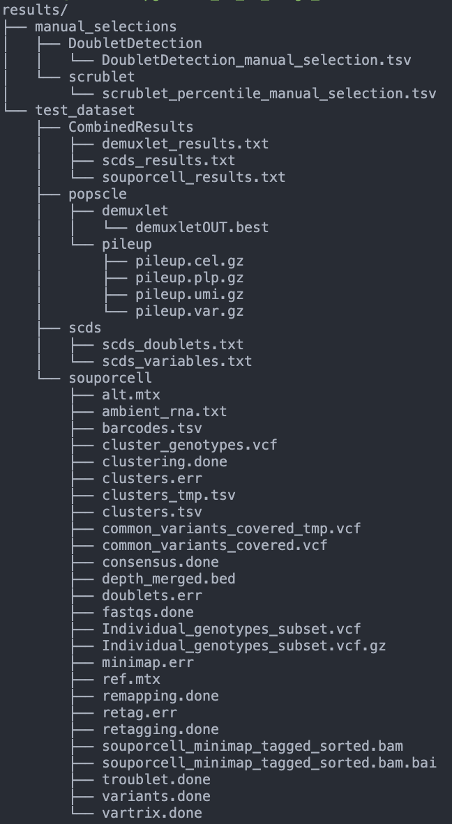
4. Once those jobs have finished running you should have a data structure similar to this:

   • There should be one manual_selections folder and one folder for each of the pools with subdirectories for each of the softwares.

     

Phase 2

Now we can run the next steps of the pipeline: DoubletDetection and Scrublet. These two softwares require that the user look at the output and decide if the thresholding is reasonable. Scrublet is sensitive to which percentile of variable genes are used for simulating and identifying doublets so, by default, we run scrublet for each pool with 4 different percentile variable genes: 80, 85, 90 and 95.

1. Let’s take a look at the jobs that will be run with a “dry run” using the same code as before:

   snakemake \
       --snakefile $SCEQTL_PIPELINE_SNAKEFILE \
       --configfile $SCEQTL_PIPELINE_CONFIG \
       --dryrun \
       --cores 1 \
       --reason
   

   • Here is the output for the dry run with one pool:

   

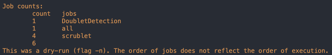
   • As you can see, there is 1 job that will be run for DoubletDetection and 4 that will be run for scrublet for our one pool (test_dataset)

2. Let’s take a look at the dag using the same code as before:

   snakemake \
       --snakefile $SCEQTL_PIPELINE_SNAKEFILE \
       --configfile $SCEQTL_PIPELINE_CONFIG \
       --dag | \
       dot -Tsvg \
           > dag2.svg
   

   • Here is the dag for the one pool that we already ran the first set of jobs for (test_dataset):

   

   • As you can see, snakemake uses dashed lines for the jobs that are completed and solid lines for the jobs that still have to be run

3. Now let’s run those jobs: the 1 DoubletDetection job and the 4 scrublet jobs using the same code as before:

   nohup \
     snakemake \
       --snakefile $SCEQTL_PIPELINE_SNAKEFILE \
       --configfile $SCEQTL_PIPELINE_CONFIG \
       --rerun-incomplete \
       --jobs 20 \
       --use-singularity \
       --restart-times 2 \
       --keep-going \
       --cluster \
           "qsub -S /bin/bash \
           -q short.q \
           -r yes \
           -pe smp {threads} \
           -l tmp_requested={resources.disk_per_thread_gb}G \
           -l mem_requested={resources.mem_per_thread_gb}G \
           -e $LOG \
           -o $LOG \
           -j y \
           -V" \
     > $LOG/nohup_`date +%Y-%m-%d.%H:%M:%S`.log &
   

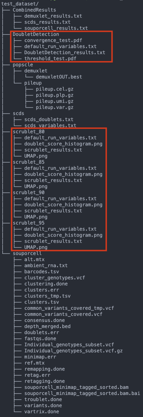
4. These jobs should not take as many resources or as long as the previous jobs so they should be done in a matter of hours. When they have completed, the data structure in your output directory should be similar to the following example with just one pool (test_dataset). The new directories and files are highlighted in red:

   

Inspection of Results

Now comes the manual part of the pipeline. Both DoubletDetection and scrublet require user input to ensure that they have correctly classified doublets.

DoubletDetection

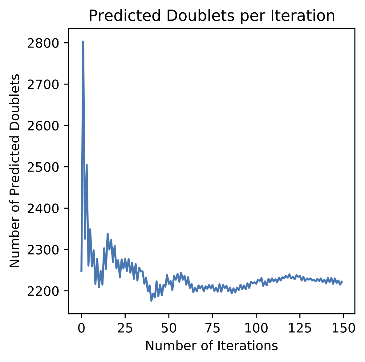
Let’s start with the DoubletDetection output. Take a look at the “convergence_test.pdf” in the DoubletDetection folder in each Pool directory. Ideally, the doublet number predicted should converge toward a common number with each iteration similar to the figure below:

Note

If you are using the smaller test dataset - provided in the singularity image - the DoulbetDetection results will not look like this - you will not have any doublets detected. This is because the dataset was so downsampled to make the dataset small for transport. You can say “PASS” anyway just to test the pipeline.

• In order to indicate whether the pool passed or failed your manual inspection, go to the “DoubletDetection_manual_selection.tsv” located in outdir/manual_selections/DoubletDetection. This is a tab separated file that has the pools in the first column and a second column header to indicate whether or not the sample passed or failed the manual inspection. For this example, this is what our tsv looks like:

  Pool	DoubletDetection_PASS_FAIL
  test_dataset

• Type “PASS” next to the pools that passed and “FAIL” next to the pools that failed the manual inspection. The pipeline will not proceed until all samples are indicated as “PASS”. Since DoubletDetection reached convergence above, we will type “PASS” into the second column of the table:

  Pool	DoubletDetection_PASS_FAIL
  test_dataset	PASS

DoubletDetection Situations Requiring Input

Sometimes DoulbetDetection does not reach convergence after 50 iterations such as below:

• In this situation, you will have to manually rerun DoulbetDetection by changing “run_DoubletDetection_manual” to True in the “DoubletDetection_manual” section of the configuration file and altering the other parameters in this section.

• Most often, DoubletDetection will reach convergence with more iterations. In this case, when we set n_iterations in the configuration yaml file to 150, we see that we do indeed reach convergence

• I have not yet encountered a pool where DoulbetDetection did not reach convergence after 150 iterations. However, if increasing the number of iterations does not enable DoubletDetection to reach convergence, try changing the phenograph parameter to True, the standard_scaling to False, p_thresh to 1e-7 and voter_thresh to 0.8 in the configuration yaml file

Note

This will cause DoubletDetection to run for much more time and use much more memory so you may have to change the memory and thread options accordingly

Note

Please note that you have to indicate the pools that need to be rerun in this section as well - a list of pools that need to be rerun should be designated in the DoubletDetection_manual_pools parameter of the configuration yaml file.

• After you have changed the parameters for a manual rerun, you can run the job with the same Snakemake commands as before. Be aware that the files in the DoubletDetection directory will be overwritten by running this manual step so move them to another directory if you want to keep them for your reference.

Scrublet

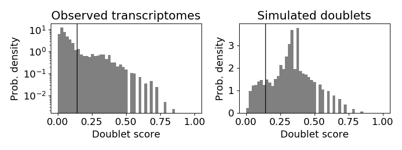
Next let’s check the scrublet results to see if the thresholding was automatically well chosen. Remember that we ran scrublet for each pool with 4 different percentile variable genes: 80, 85, 90 and 95. Take a look at the “doublet_score_histogram.png” in each of the scrublet directories in each of the pool directories. You want to see that the threshold that was automatically selected nicely separates a bimodal distribution of simulated doublets like below:

• In order to identify which scrublet results should be used for downstream analyses, you need to decide which percentile variable gene threshold resulted in the best simulated doublet bimodal distribution with an effectively set threshold and provide that information in the outdir/manual_selections/scrublet/scrublet_percentile_manual_selection.tsv file. For this example, the contents of our scrublet_percentile_manual_selection.tsv look like this:

  Pool	scrublet_Percentile
  test_dataset

• Enter the percentile variable gene threshold number that resulted in the best bimodal distribution and effectively selected a threshold for the doublet score into the second column of scrublet_percentile_manual_selection.tsv. In our case, the best distribution and threshold selection was for 95th percentile variable genes so we enter the number 95 next to our pool:

  Pool	scrublet_Percentile
  test_dataset	95

• If you are not happy with any of the scrublet results, leave the second column of that row empty and use the manual rerun function. The pipeline will not proceed until all pools have a value in the second column.

Scrublet Situations Requiring Input

Occasionally, scrublet does not choose an appropriate threshold so it will have to be set manually. Here is an example figure from that situation for “Pool7”:

• In this situation, you would want to find the percentile level that results in the best bimodal distribution of the simulated doublets and then rerun with different parameters by setting “run_scrublet_manual” to True in the configuration yaml file and putting changing the other parameters in the scrublet_manual section of the configuration yaml. For this example, the best bimodal distribution of simulated doublets was for the 95th percentile of variable genes:

• As you can see, the distribution is still very similar to the previous figure, but the separation between the two distributions is a bit clearer. However, the threshold selected by scrublet still doesn’t seem quite right and should probably be closer to ~0.21

• Therefore, to set a better threshold to select doublets for this pool, you would change the following parameters in the scrublet_manual section of the configuration yaml file:

run_scrublet_manual: True
scrublet_manual_threshold_pools: [Pool7]
scrublet_manual_threshold_percentiles: [95]
scrublet_manual_threshold_thresholds: [0.21]

• If you had two pools that you wanted to rerun, say Pool7 and Pool13 but you wanted to use 95 percent variable genes and 0.21 doublet score for Pool7 but 85 percent variable genes and 0.25 doublet score for Pool13, your parameters would look like this:

run_scrublet_manual: True
scrublet_manual_threshold_pools: [Pool7,Pool13]
scrublet_manual_threshold_percentiles: [95,85]
scrublet_manual_threshold_thresholds: [0.21,0.25]

• Then you would run the job with the same Snakemake commands as before. Be aware that if you use one of the variable gene percentiles originally used (80, 85, 90 or 95), the contents of that directory will be overwritten by this manual step. If you want to keep those files for your records, move them to a new directory.

Last run

Ok, done with the hard part. Now that you have decided that DoubletDetection and scrublet effectively identified doublets for each of your pools, make sure that you have all the rows of the second column in the manual_selections files filled in with appropriate values. Now the pipeline will proceed with the final steps of merging the results, identifying final cell types and producing QC figures. Let’s make sure that is what will be run by doing a dry run:

snakemake \
    --snakefile $SCEQTL_PIPELINE_SNAKEFILE \
    --configfile $SCEQTL_PIPELINE_CONFIG \
    --dryrun \
    --cores 1 \
    --reason

• Here is the output for the dry run with one pool:

1. Let’s take a look at the dag for this last Snakemake run using the same Snakemake command:

snakemake \
  --snakefile $SCEQTL_PIPELINE_SNAKEFILE \
  --configfile $SCEQTL_PIPELINE_CONFIG \
  --dag | \
  dot -Tsvg \
      > dag3.svg

• As you can see, the first jobs that will be run are jobs to check whether the your input is complete, then the results from each of the softwares will be combined into a single tab separated file, the individual IDs will be added for the souporcell results (which just identifies clusters by default but doesn’t assign individual IDs to them). Then a few final checks will be done before producing the final QC figures.

1. Let’s run the final steps of the pipeline with the same Snakemake command as before:

   nohup \
     snakemake \
       --snakefile $SCEQTL_PIPELINE_SNAKEFILE \
       --configfile $SCEQTL_PIPELINE_CONFIG \
       --rerun-incomplete \
       --jobs 20 \
       --use-singularity \
       --restart-times 2 \
       --keep-going \
       --cluster \
           "qsub -S /bin/bash \
           -q short.q \
           -r yes \
           -pe smp {threads} \
           -l tmp_requested={resources.disk_per_thread_gb}G \
           -l mem_requested={resources.mem_per_thread_gb}G \
           -e $LOG \
           -o $LOG \
           -j y \
           -V" \
     > $LOG/nohup_`date +%Y-%m-%d.%H:%M:%S`.log &
   

   • The QC figures use Seurat to merge and process the data from each pool so the amount of memory that will be needed for this step will be dependent on the number of pools in your dataset. Like all other steps, depending on the number indicated for --restart-times, this step will rerun with more memory if it fails.

2. Following completion of these last steps, your final directory structure should be similar to the following with the new directories and files highlighted in red:

   

3. In addition, you will have an additional directory called QC_figures:

   

4. Finally, let’s create a report that includes all of our results and some pipeline metrics:

   nohup \
     snakemake \
       --snakefile $IMPUTATION_SNAKEFILE \
       --configfile $IMPUTATION_CONFIG \
       --report demultiplexing_report.html
   

   This will generate an html report that includes figures and pipeline metrics called demultiplexing_report.html. The report generated for this testa dataset is available here.

Checking the Output

Each of the figures generated by this pipeline are included in the demultiplexing_report.html and it can therefore be used to check the results of the pipeline. These figures will be used for discussion with members of the sceQTL-Gen Consortium to identify appropriate filtering thresholds for your dataset. In addition, we include the locations of each of these files in your directories for each of the figures below.

1. First, we can check the assignments of individuals to the clusters identified by souporcell. Those results are available in the Souporcell Genotype Correlations folder in the demultiplexing_report.html and are located in each pool directory in the souporcell/genotype_correlations/ directory. Take a look at the pearson_correlation.png which should have the pearson correlation between each genotypes from each cluster identified by souporcell and the genotypes of the individuals that were in that pool. Your figure should look similar to: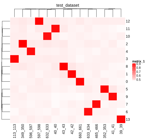

   

   • As you can see, each individual (x-axis) is highly correlated with one souporcell cluster (y-axis). Double check that this is true for all of your pools as well.

   • The final key used for assigning individuals to clusters is also in this directory: Genotype_ID_key.txt. Here are the contents of this file for this pool:

   Genotype_ID	Cluster_ID	Correlation
   113_113	3	0.9348012632264568
   349_350	2	0.9417452138320714
   352_353	5	0.9373211752184873
   39_39	13	0.9287080212127417
   40_40	11	0.92255735671204
   41_41	9	0.9247177216756595
   42_42	1	0.93031509740497nn
   43_43	8	0.9452410331923875
   465_466	7	0.9231136486662362
   596_597	4	0.9207862818303282
   597_598	12	0.9352949932462498
   632_633	10	0.913163676189583
   633_634	6	0.9166092993097202
   660_661	0	0.9359090212760529

   • This file will be used to substitute the souporcell cluster IDs with the individual IDs

2. Next, let’s see how many cells were classified as “singlet” and the number of individuals that we were able to detect. You will find a figure (expected_observed_individuals_classifications.png) with two barplots demonstrating these metrics across all the pools in the Number Individuals Summary folder in the demultiplexing_report.html and in the QC_figures directory locally:

   

3. In addition, there is another barplot figure that demonstrates the nubmer of droplets assigned to each individual and how many were classified as “doublets” or “unassigned”. You will find a barplot of this data(DropletType_Assignment_BarPlot.png) in Number Individuals Summary folder in the demultiplexing_report.html and in the CombinedResults folder locally in each Pool. These are the final assignments for each droplet after intersecting the results from all of the softwares.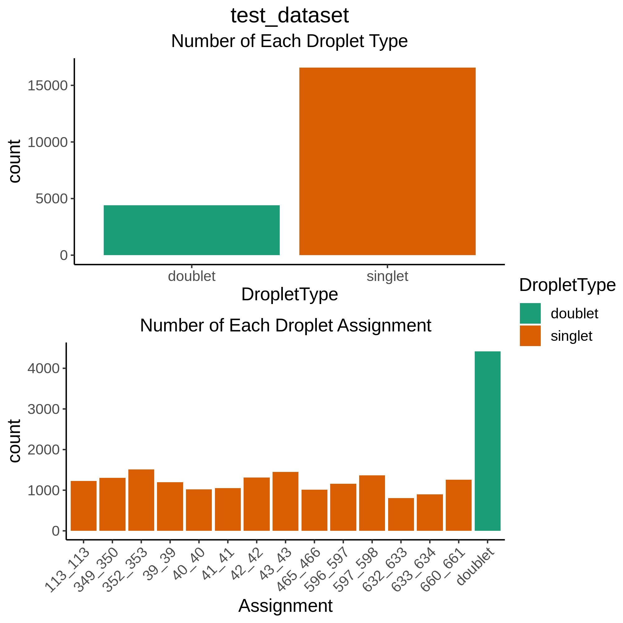

   

   • As you can see, for this intersectional method, we identified ~4,000 doublets and ~1,000 singlets per individual. The doublet rate is a bit higher than anticipated (20% instead of 16%) but we wanted to be more conservative with singlet selection for this consortium to remove noise for cell classification (working group 2) and eQTL detection (working group 3).

   • Please be aware that if you have individuals in a pool that were not genotyped, they will be called doublets. So in pools where not all individuals were genotyped you will see far more doublets than anticipated for the number of droplets that were captured. Here is an example where 15 individuals were pooled together but, due to various reasons, the genotype data was only available for 11 of those individuals, resulting in almost half the droplets being called “doublets”:

   

   • Once you calculate that you expect ~3,200 doublets for this capture and ~1,000 cells per individual with 4 individuals who were not genotyped, we expect ~7,200 droplets to be classified as doublets.

   • If you find that the results in this figure are unanticipated (ie you have far more or far fewer singlets or doublets than expected), that would be a really good indication that either there is something strange about this pool (ie most droplets didn’t contain cells) or that one or more of the softwares need to be rerun with different parameters. You can reach out to us by opening an issue if you find that this is the case and we can troubleshoot with you.

4. Now let’s check the contents of the QC figures. A number of QC metrics have been plotted and are in the QC folder in the demultiplexing_report.html and saved in the QC_figures directory locally. As you can see, there are a number of files and figures have been generated. The single cell counts have been stored in a Seurat object and saved at various stages of processing:

seurat_object_all_pools_all_barcodes_all_metadata.rds

has all the droplets from all pools and also has each of the software assignments in the meta.data slot. The meta.data slot of the seurat object has all the droplets as rows and the following columns:

• orig.ident: Name for the project. This will be “SeuratProject” by default

• nCount_RNA: nUMIs per cell

• nFeature_RNA: Number of genes per cell

• Barcode: Original barcode ID; Note that this will be different from the rownames as seurat automatically changes the barcode names when multiple pools are merged together so that there are no issues with replicate barcode names across pools

• demuxlet_nSNP: The number of SNPs used for each droplet to determine the cell assignment for demuxlet

• demuxlet_DropletType: The droplet type assignment from demuxlet (singlet, doublet, unassigned)

• demuxlet_Assignment: The droplet individual assignment (individual ID, doublet or unassigned)

• demuxlet_SingletLLK: The log likelihood for the best singlet assignment from demuxlet

• demuxlet_DoulbetLLK: The log likelihood for the best doublet assignment from demuxlet

• demuxlet_DiffLLK: The difference of the singlet and doublet log likelihoods demuxlet (this ratio is used to call whether a droplet is a singlet or a doublet)

• souporcell_DropletType: The droplet type assignment from souporcell (singlet, doublet, unassigned)

• souporcell_Assignment: The droplet individual assignment from souporcell (individual ID, doublet or unassigned)

• souporcell_LogProbSinglet: The log probability of the best singlet assignment from souporcell

• souporcell_LogProbDoublet: The log probability that the droplet is a doublet from souporcell

• scrublet_DropletType: The droplet type assignment from scrublet (singlet, doublet, unassigned)

• scrublet_Scores: The scrublet doublet scores

• scds_score: The doublet score assigned by scds

• scds_DropletType: The droplet type assignment from scds (singlet, doublet, unassigned)

• DoubletDetection_DropletType: The droplet type assignment from DoubletDetection (singlet, doublet, unassigned)

• Pool: Pool name that droplet was collected in

seurat_object_all_pools_all_barcodes_final_assignments.rds

has all the droplets from all pools and includes some metadata including the final droplet types and cell assignments from the intersectional method

• orig.ident: Name for the project. This will be “SeuratProject” by default

• nCount_RNA: nUMIs per cell

• nFeature_RNA: Number of genes per cell

• Barcode: Original barcode ID; Note that this will be different from the rownames as seurat automatically changes the barcode names when multiple pools are merged together so that there are no issues with replicate barcode names across pools

• Assignment: The droplet individual assignment from the intersectional method (individual ID, doublet or unassigned)

• DropletType: The droplet type assignment from the intersectional method (singlet, doublet or unassigned)

• Pool: Pool name that droplet was collected in

seurat_object_all_pools_singlet_barcodes_final_assignments.rds

only contains singlets as identified with the intersectional method file and has the same metadata as the last object as well as mitochondrial and ribosomal percent

• orig.ident: Name for the project. This will be “SeuratProject” by default

• nCount_RNA: nUMIs per cell

• nFeature_RNA: Number of genes per cell

• Barcode: Original barcode ID; Note that this will be different from the rownames as seurat automatically changes the barcode names when multiple pools are merged together so that there are no issues with replicate barcode names across pools

• Assignment: The droplet individual assignment from the intersectional method (individual ID, doublet or unassigned)

• DropletType: The droplet type assignment from the intersectional method (singlet, doublet or unassigned)

• Pool: Pool name that droplet was collected in

• percent.mt: Percent of genes that are mitochondrial per droplet

• percent.rb: Percent of genes that are ribosomal per droplet

Uploading Data

Upon completing the Demultiplexing and Doublet Removal pipeline, please upload your seurat_object_all_pools_all_barcodes_all_metadata.rds and demultiplexing_report.html to the shared own cloud. This will be the same link you used to upload your data at the end of the SNP Imputation pipeline. However, if you have not already organized a link for data upload, contact Marc Jan Bonder at bondermj @ gmail.com to get a link to upload the seurat_object_all_pools_all_barcodes_all_metadata.rds and demultiplexing_report.html. Be sure to include your dataset name as well as the PI name associated to the dataset. This link will also be used for data upload WG2 results.

Important

Please note you can’t change filenames after uploading!

Next Steps

A number of QC figures of the singlet droplets have also been produced. These can be used to discuss possible QC thresholds with the WG1 and before final QC filtering. Let’s move to the QC Filtering Section to discuss the figures produced and next next steps for additional QC filtering.